Tập tin:Solar AM0 spectrum with visible spectrum background (en).png
Kích thước hình xem trước: 800×494 điểm ảnh. Độ phân giải khác: 320×198 điểm ảnh | 640×395 điểm ảnh | 1.024×632 điểm ảnh | 1.280×790 điểm ảnh | 1.882×1.162 điểm ảnh.
Tập tin gốc (1.882×1.162 điểm ảnh, kích thước tập tin: 181 kB, kiểu MIME: image/png)
Tập tin này từ Wikimedia Commons. Trang miêu tả nó ở đấy được sao chép dưới đây. Commons là kho lưu trữ tập tin phương tiện có giấy phép tự do. Bạn có thể tham gia. |
.png?uselang=vi)
Miêu tả
| Miêu tả |
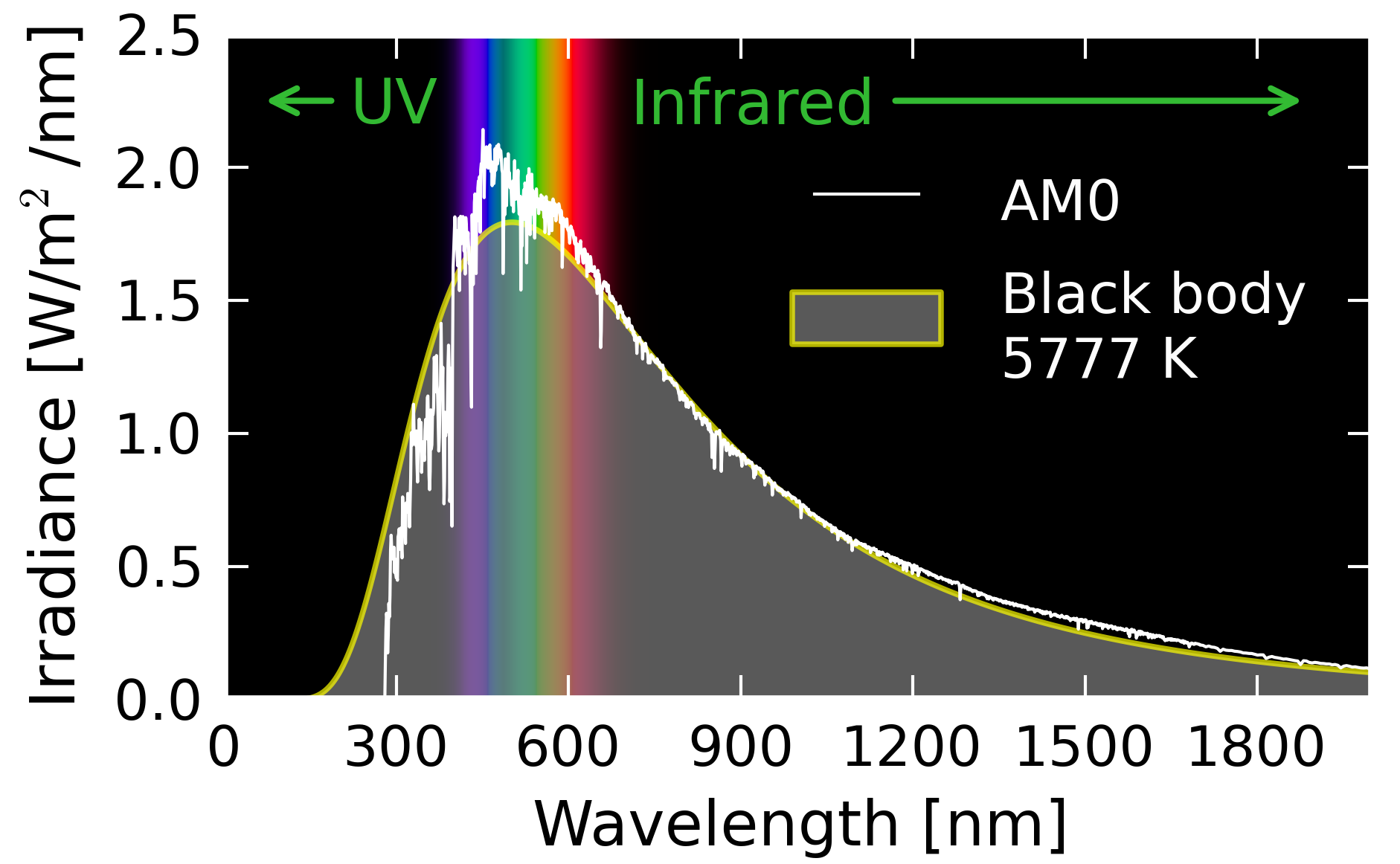
English: Solar AM0 (Air Mass Zero) spectrum (Chris A. Gueymard 2002) as included in SMARTS 2.95, together with a blackbody spectrum for 5777 kelvin and solid angle 2.16e-5*π steradian for the source (the solar disk). The visible region of the electromagnetic spectrum is shown using the CIE visible spectrum as implemented in ColorPy by Mark Kness (2008). Figure with English labels. |
| Ngày | |
| Nguồn gốc |
Tác phẩm được tạo bởi người tải lên This plot was created with Matplotlib. |
| Tác giả | Danmichaelo |
| Phiên bản khác | Version with Norwegian labels |
.png)
| Source |
|---|
#encoding=utf8

import matplotlib
from matplotlib import rc
from matplotlib import pyplot as plt
import numpy as np

rc('lines', linewidth=0.5)
rc('font', family='sans-serif', size=10)
rc('axes', labelsize=10)
rc('xtick', labelsize=9)
rc('ytick', labelsize=9)

golden_mean = (np.sqrt(5)-1.0)/2.0
inches_per_cm = 1.0/2.54
fig_width = 8 * inches_per_cm
fig_height = golden_mean * fig_width
fig = plt.figure(figsize = [fig_width, fig_height])

from colorpy import ciexyz, colormodels

Fs = 2.16e-5 * np.pi;   # Geometrical factor of sun as viewed from Earth
h = 6.63e-34;           # Boltzmann const. [Js]
c = 3.e8;               # speed of light [m/s]
q = 1.602e-19;          # electron charge [C]

def blackbody(wvlgth, temp):
    # per nanometer 1e-9:
    fac = (2 * Fs * h * c**2) / ((wvlgth * 1.e-9)**5)
    return fac / (np.exp(1240./(wvlgth*8.62e-5*temp)) - 1) * 1.e-9

def draw_vis_spec(ax, ymax):
    spectrum = ciexyz.empty_spectrum()[:,0]
    (num_wl,) = spectrum.shape
    rgb_colors = np.empty((num_wl, 3))
    for i in xrange (0, num_wl):
        xyz = ciexyz.xyz_from_wavelength(spectrum[i])
        rgb = colormodels.rgb_from_xyz(xyz)
        rgb_colors [i] = rgb
    rgb_colors /= np.max(rgb_colors) # scale to make brightest rgb value = 1.0

    num_points = len(spectrum)
    for i in xrange (0, num_points-1):
        x0 = spectrum[i]
        x1 = spectrum[i+1]
        y0 = 0.0
        y1 = ymax
        poly_x = [x0, x1, x1, x0]
        poly_y = [y0, y0, y1, y1]
        color_string = colormodels.irgb_string_from_rgb(rgb_colors [i])
        ax.fill(poly_x, poly_y, color_string, edgecolor=color_string)

ax = fig.add_subplot(111)

frame = ax.get_frame()
frame.set_facecolor('black')
xmax = 2000
ymax = 2.5

# Visible spectrum:

draw_vis_spec(ax, ymax)

# Blackbody:

temp = 5777
x = np.arange(100, 2000)
y = blackbody(x, temp)
y[-1] = 0.
ax.fill(x, y, '0.5', alpha = 0.7, linewidth = 0.9, edgecolor='yellow', label = 'Black body\n%d K' % temp)

# AM0 spectrum:

d = np.loadtxt('smarts295.ext.txt', skiprows = 1)
x = d[:,0]
y = d[:,1]
y[0] = 0.
y[-1] = 0.
ax.plot(x, y, color='white', linewidth=0.5, label = 'AM0')
ax.set_xlim(0, xmax)
ax.set_xticks(np.arange(0, 1999, 300))
ax.set_ylim(0, ymax)

# Tweak, tweak and annotate:

texty = 2.25
ax.annotate('UV', xy = (50,texty), xytext = (230,texty), xycoords = 'data',
        horizontalalignment='left', verticalalignment='center', color='#33bb33',
        arrowprops = dict(arrowstyle='->', color='#33bb33'))
#ax.annotate('Synlig', xy=(400,texty), xycoords='data',
#        horizontalalignment='left', verticalalignment='center', color='white')
ax.annotate(u'Infrared', xytext = (720,texty), xy = (1900,texty), xycoords = 'data',
        horizontalalignment='left', verticalalignment='center', color='#33bb33',
        arrowprops = dict(arrowstyle='->',color='#33bb33'))

leg = ax.legend(loc='upper right', frameon=False, bbox_to_anchor = (1.0, 0.90) )
txts = leg.get_texts()
for txt in txts:
    txt.set_color('white')
    txt.set_fontsize(9)

ax.tick_params(color='white', labelcolor='black')
for spine in ax.spines.values():
    spine.set_edgecolor('white')
    spine.set_linewidth(1.4)

fig.subplots_adjust(left=0.16, bottom = 0.19, right=0.98, top=0.96)

ax.set_xlabel(u'Wavelength [nm]')
ax.set_ylabel(u'Irradiance [W/m$^2$/nm]')
fig.savefig('Solar AM0 spectrum with visible spectrum background (en).png',dpi=600)
|
Giấy phép
| Tôi, người giữ bản quyền của tác phẩm này, chuyển tác phẩm này vào phạm vi công cộng. Điều này có giá trị trên toàn thế giới. Tại một quốc gia mà luật pháp không cho phép điều này, thì: Tôi cho phép tất cả mọi người được quyền sử dụng tác phẩm này với bất cứ mục đích nào, không kèm theo bất kỳ điều kiện nào, trừ phi luật pháp yêu cầu những điều kiện đó. |
Lịch sử tập tin
Nhấn vào ngày/giờ để xem nội dung tập tin tại thời điểm đó.
| Ngày/giờ | Hình xem trước | Kích cỡ | Thành viên | Miêu tả | |
|---|---|---|---|---|---|
| hiện tại | 20:32, ngày 16 tháng 5 năm 2012 | | 1.882×1.162 (181 kB) | Danmichaelo |
Trang sử dụng tập tin
Có 1 trang tại Wikipedia tiếng Việt có liên kết đến tập tin (không hiển thị trang ở các dự án khác):
.png)